Bootstrapping Time Series
We have a “compare” feature in our product at work. Here’s what that looks like:
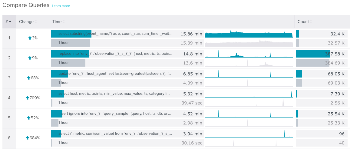
That picture shows the change in total query execution time for two time ranges. The percent change is calculated against the sums of points in the “Time” (execution time) time series.
You’ll notice that a couple of those queries have huge change percents. Over 600%! There are also a few spikes in the time series. Those outliers can really mess things up. Imagine what happens when a database server stalls up: nothing gets done for a short period of time and every query’s execution time goes up. If you’re looking for changes during a period that had a stall, you’re out of luck. All of your percents will probably be really high because of that stall.
What would make this feature a lot better is some notion of statistical significance. If there’s a large change, you should be able to know if it’s because of an actual change and not an unlucky combination of points. This is what hypothesis tests are used for in statistics.
Usually with hypothesis tests, you have a bunch of samples that come from a single population that you use to create a model for the population. Then, you take a brand new sample that you know almost nothing about and try to see if it fits within the model you created before. Unfortunately, we can’t take the same approach in this case because we only have one prior sample.
That’s where bootstrapping comes in.
Bootstrap
Bootstrapping is a technique that lets you generate new samples from an existing sample. It relies on sampling with replacement. Bootstrapping is not a new technique. Bradley Efron proposed it in the late 1970s. I heard it didn’t gain much use because of its high computational requirements. Now that computers are powerful enough, bootstrapping is getting more popular.
Suppose you had a 5-element array and its sum:
[1, 2, 3, 4, 5] => 15
Sampling with replacement can give you results like this. Notice how some of the sums are smaller than the original 15, and some are larger.
[1, 2, 2, 2, 2] => 9
[4, 4, 3, 1, 2] => 14
[2, 4, 4, 2, 4] => 16
[1, 3, 3, 5, 2] => 14
[5, 1, 3, 2, 3] => 14
[4, 5, 3, 3, 5] => 20
[3, 2, 2, 2, 2] => 11
[3, 1, 3, 1, 3] => 11
[2, 4, 2, 3, 5] => 16
[3, 4, 1, 2, 5] => 15
When you run that a hundred times and plot a histogram of the sums…
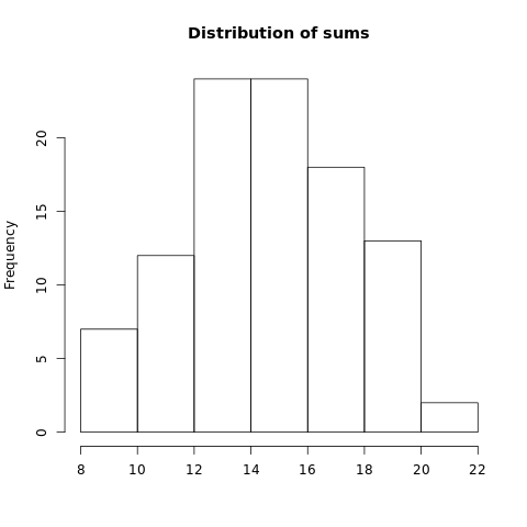
…you get a nice distribution! You can do a lot of cool things with that distribution, like calculate confidence intervals. This is what you can use for hypothesis tests.
Examples
These examples all use sums of time series. Points of series 1 are sampled with replacement to generate a distribution of sums. The sum of series 2 is compared against that distribution to check for significance.
In this first example, both time series are based on Math.random() with an average around 3, but
series 1 has a value of 80 at index 25.
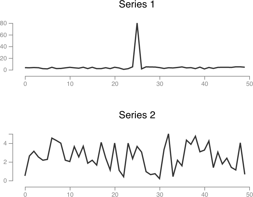
Series 1 sum: 239.29
Series 2 sum: 126.29
Percent change: -47.22%
Significant: FALSE
Series 2’s sum is 47% lower, but this change is not significant. Clearly our spike had a big impact on the series 1 sum.
This next example is real data. These time series represent error counts for a single query. The percent change tells us that the number of errors in the second time range went down by almost a half. I wouldn’t put too much faith into that number, though. Bootstrapping tells us this change isn’t significant.
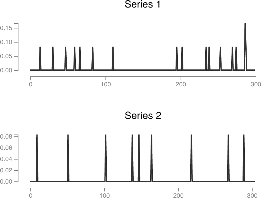
Series 1 sum: 1.42
Series 2 sum: 0.75
Percent change: -47.06%
Significant: FALSE
Finally, we’ll go back to a randomly generated example. These are also using the same formula, but series 2 is shifted up a little bit.
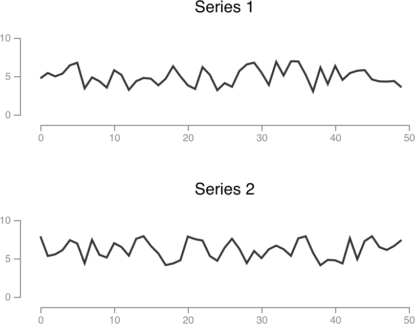
Series 1 sum: 248.63
Series 2 sum: 307.89
Percent change: 23.83%
Significant: TRUE
Bootstrapping tells us this change is significant. Cool!
I’ve only covered sums in this post, but this technique can be applied with any kind of aggregation. You can create distributions of averages, quantiles, minimums, maximums… anything that can take advantage of sampling with replacement. I think bootstrapping has lots of potential, and it’s really easy to implement!
EDIT: The takeaway in the original post may not have been clear. This approach is not a new way of detecting changes without outliers or anything like that. I don’t even think there’s anything wrong with the percent change itself. The main takeaway is that a single number like the percent change can be affected by outliers and typical variability of systems. A number like that is hard to interpret by itself. By bootstrapping, you can create some sort of confidence or significance indicator that can help you interpret results. For example, an average is much more useful if you also had the standard deviation because the standard deviation gives you an idea of what the spread of the data is like. The time series example I showed in this post uses bootstrapping to give you a better idea about whether or not there is an actual, significant change in a time series.
Example code
var series1 = []; // This contains the time series values of the previous time range.
var series2 = []; // This contains the time series values of the current time range.
var series1Sum = sum(series1);
var series2Sum = sum(series2);

// Bootstrapping requires sampling with replacement.

var bootstrappedSums = []; // Resampled sums
var rounds = 1000; // Total bootstrap rounds

for (var i = 0; i < rounds; i++) {
  var sum = 0;

  // Sample series1.length times from series1 with replacement
  for (x in series1) {
    var index = Math.floor(Math.random() * series1.length);
    sum += series1[index];
  }

  bootstrappedSums.push(sum);
}

// Sort the sums
bootstrappedSums.sort(function (a, b) {
  return a - b;
});

// Get the boundaries
var bootstrapLow = bootstrappedSums[0]; // can also use a low quantile
var bootstrapHigh = bootstrappedSums[rounds - 1]; // can also use a high quantile

// Check for significance
var significant = "FALSE";
if (series2Sum < bootstrapLow || series2Sum > bootstrapHigh) {
  // series2 sum is outside of the expected range
  significant = "TRUE";
}